Types of SQL Joins: Inner, Left, Right, and Full

For data engineers and data scientists, SQL is valuable expertise. All modern data warehouses as well as data or delta lakes have SQL interfaces. Understanding how an SQL query is executed can help you write fast and economical queries.

Once you understand SQL concepts like join and window, you will intuitively understand the similar APIs in Spark, Pandas, or R. After all, SQL is one of the ancient programming languages that are still best for what they were invented for (another such example is C for system programming).

SQL first appeared in 1974 for accessing data in relational databases, and its latest standard was published in 2016. It is a declarative language (i.e. a programmer specifies what to do, and not how to do it) with strong static typing.

SQL Join is one of the most common and important operations to merge data with different attributes (or columns) from different sources (or tables). In this article, you will learn about various kinds of SQL joins and best practices to write efficient joins on large tables.

Types of SQL Joins

SQL JOIN operations are used to combine rows from two or more tables, and are of two types:

• Conditional Join: Combine rows based on a condition over one or more common columns (typically primary or foreign keys). There are 4 types of conditional joins: inner, left, right, and full.

• Cross Join: Cartesian Product of two tables.

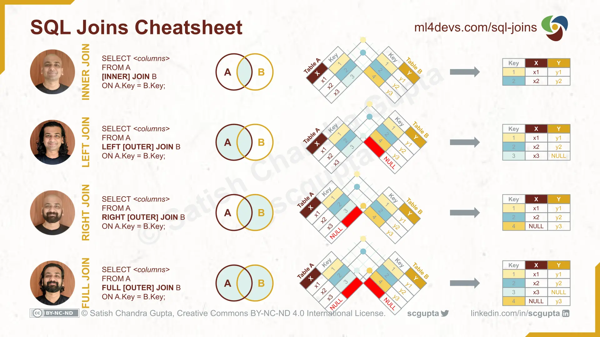
INNER JOIN

An Inner Join produces a row combining a row from both tables only if the key is present in both tables.

For example, if you had run two marketing campaigns on different channels that captured potential customer info in two tables:

• Table A: Name and phone number
• Table B: Name and email

Table A:
      Name      |      Phone
----------------+-----------------
 Warren Buffett | +1-123-456-7890
 Bill Gates     | +1-987-654-3210

Table B:
      Name      |      Email
----------------+-----------------
 Bill Gates     | bgates@live.com
 Larry Page     | lpage@gmail.com

You can find all customer leads for which you have both their phone number and email address using an Inner Join:

1
2
3
4

SELECT A.Name, A.Phone, B.Email
FROM A
INNER JOIN B
ON A.name = B.name;

The word INNER is optional and you can omit it if you want. The result will be:

      Name      |      Phone      |      Email
----------------+-----------------+-----------------
 Bill Gates     | +1-987-654-3210 | bgates@live.com

LEFT OUTER JOIN

A Left Join returns all rows from the left table and the matched rows from the right table.

Say, your sales team decides to reach out to all customer leads over the phone, but, if possible, wants to follow up by email too. With a Left Join, you can create a list of customers where you have their phone numbers for sure but may also have their email:

1
2
3
4

SELECT A.Name, A.Phone, B.Email
FROM A
LEFT OUTER JOIN B
ON A.name = B.name;

The word OUTER is optional and you can omit it if you want. The result will be:

      Name      |      Phone      |      Email
----------------+-----------------+-----------------
 Warren Buffett | +1-123-456-7890 |      null
 Bill Gates     | +1-987-654-3210 | bgates@live.com

RIGHT OUTER JOIN

A Right Join returns all rows from the right table and the matched rows from the left table.

Say, you want the opposite: all customers with an email address and, if possible, their phone numbers too:

1
2
3
4

SELECT B.Name, A.Phone, B.Email
FROM A
RIGHT OUTER JOIN B
ON A.name = B.name;

The word OUTER is optional and you can omit it if you want. The result will be:

      Name      |      Phone      |      Email
----------------+-----------------+-----------------
 Bill Gates     | +1-987-654-3210 | bgates@live.com
 Larry Page     |      null       | lpage@gmail.com

FULL OUTER JOIN

A Full Join returns all rows from both tables matching them whenever possible.

Say, you want to have a consolidated list of all customers having a phone number or email address or, if possible, both:

1
2
3
4
5
6
7
8
9

SELECT
  CASE
    WHEN A.Name IS NOT NULL THEN A.Name
    ELSE B.Name
  END AS Name,
  A.Phone, B.Email
FROM A
FULL OUTER JOIN B
ON A.name = B.name;

The word OUTER is optional and you can omit it if you want. In some databases, a simple SELECT * might work and you will not need that CASE statement. The result will be:

      Name      |      Phone      |      Email
----------------+-----------------+-----------------
 Warren Buffett | +1-123-456-7890 |      null
 Bill Gates     | +1-987-654-3210 | bgates@live.com
 Larry Page     |      null       | lpage@gmail.com

Here is a cheatsheet for all 4 conditional joins:

CROSS JOIN

SQL Cross Join is the Cartesian Product of two tables. It pairs each row of the left table with each row of the right table.

Say, you have a table CarType with 7 rows having values: Sedan, Hatchback, Coupe, MPV, SUV, Pickup Truck, and Convertible.

And you also have a table Color with 5 rows: Red, Black, Blue, Silver Grey, and Green.

A Cross Join between the two will generate a table with 35 rows having all possible combinations of car types and colors:

1
2
3

SELECT *
FROM CarType
CROSS JOIN Color;

I have not come across any use of a Cross Join in a data analytics or data science project.

Understanding SQL Joins

Not all SQL queries are created equal. Join is typically a costly operation. Since Online Analytics Processing (OLAP) applications process a huge amount of data, optimized SQL queries can save you time and money.

Most data warehouses report the query execution plan and costs of various parts after running your query. Examining it can help you in optimizing your storage as well as the query.

Intuition from Relational Algebra

The query plan for a SQL Join has at least the following Relational Algebra operators:

• Projection (Π): the subset of columns from tables. This corresponds to the column list after the SELECT keyword in the query.

• Selection (σ): the subset of rows filtered by a condition. This comes from conditions defined in the WHERE clause in the query.

• Join (⋈): the join between the tables coming from the JOIN operation.

The key to optimizing a SQL Join query is to minimize the sizes of the tables fed to the Join (⋈) operator. Following best practices are designed to do precisely that.

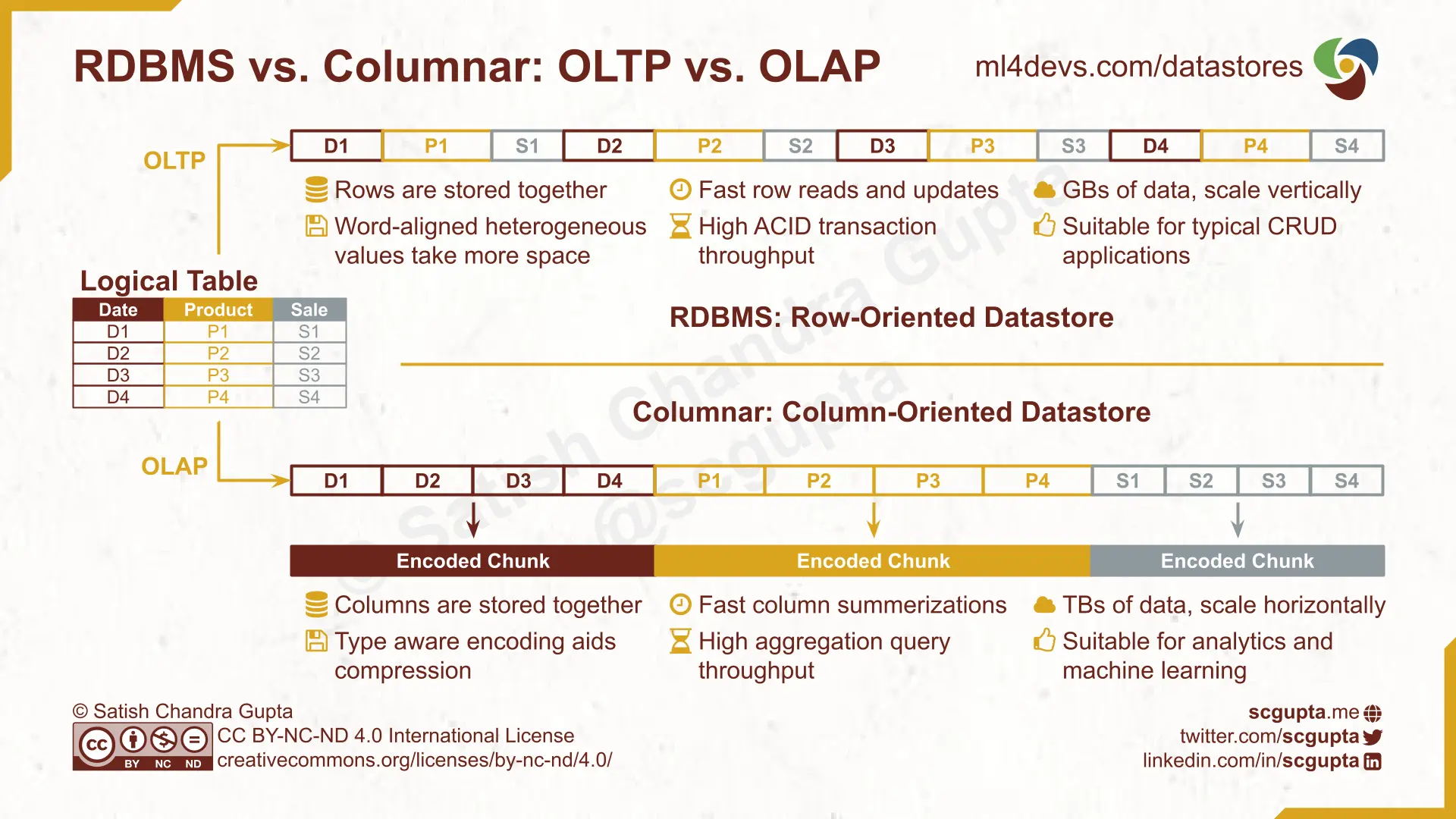
1. Select only the columns you need

Data warehouses are Columnar databases, i.e., values in a column are stored together (in RDBMS, the rows are stored together). Therefore, SELECT * is a particularly bad idea.

2. Make filtering fast by partitioning and clustering

Think about typical WHERE clauses you will be using, and identify the columns used most other for the filtering. Depending upon your database, do whichever of the following is possible:

• Partition the tables on a commonly used column that splits data evenly (e.g. timestamp, date).

• Clustering on columns orders the data within a partition. If you defined multiple clustering columns, the data is stored in nested sort order. This colocates the data that matches your common filtering conditions.

3. Carefully order the conditions in the WHERE clause

In the WHERE clause, use the conditions on partitioned and clustered columns first, as those will run faster.

Order the rest of the conditions such that the one that filters out the most rows comes first. That way, each condition will trim down the maximum number of rows possible.

4. Trim down the rows as much as possible

The more rows the left and right table have, the longer it will take to match the keys in the join. You can reduce the number of rows by:

• Filtering the data as early as possible: whenever possible, filter a table in a sub-query before the join instead of after the join.

• Aggregating the data as early as possible: aggregations reduce the number of rows drastically, so whenever possible, do an aggregation before a join instead of after the join.

5. Do the JOIN as late as possible

This is obvious, but I must reiterate the point: do everything possible to reduce the size of the left and right tables before feeding them to the JOIN operation.

Summary

SQL Joins are common operations in data analytics and data science. You learned about the inner, left, right, and full joins, and also the best practices for optimizing SQL Join queries.